One of the most important factors in evaluating an oil reservoir is porosity, permeability & water saturation cutoff. These are 3 very important factors to assess whether an oil reservoir is economically viable or not.
- Cutoff is used to determine the "net pay" (the portion of a reservoir that can be economically recovered) and "reservoir rock". Reservoir rock is rock with sufficient porosity/permeability to allow hydrocarbons to migrate to the wellbore (meeting porosity & permeability cutoff values). If the reservoir rock meets the water saturation cutoff value (the highest Sw / Swe value that still produces hydrocarbons), the reservoir rock is considered net pay.
- Typical porosity & permeability cutoff values are around 5% in conventional oil reservoirs. Therefore, only the portion of the geological formation with a porosity greater than this value is considered in the reservoir's recovery potential forecast. It is implicitly understood that geological intervals with higher porosity have better permeability, although there are some exceptions (usually due to fractures).
In the paper, the two authors used GAN to create unconditional simulations of Ketton limestone and Maules (Australia) sandstone models. This post focuses on the processing of the Ketton limestone dataset.
GAN, a deep learning model belonging to the generative model group, is a model capable of generating data, created with the expectation of producing highly accurate systems that require less human intervention in the training process.
GAN consists of two networks: Generator G(z) maps samples obtained from a multivariate standard normal distribution to an image x, and Discriminator D(z) assumes the role of a classifier to distinguish between the generated simulations x ~ G(z). Both networks are trained in an alternating two-step process to optimize the min-max objective function:

One of the convenient points of the paper is that the notebook file and pre-trained GAN models are available. You can view them at the author's Github repo: https://github.com/LukasMosser/geogan
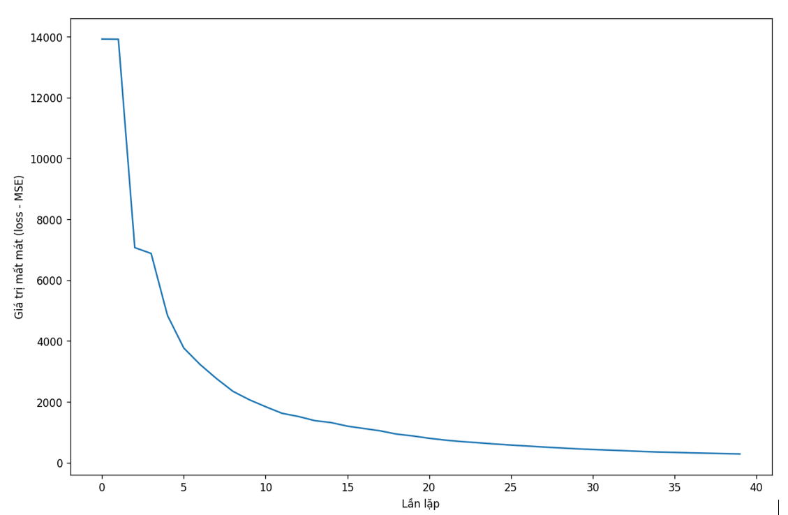
Some results after putting the notebook on Google Colab and running:

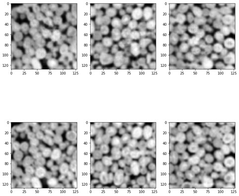
Compare the data by visualizing the conditioned image with the image from GAN:
x_cond = generator (cond.zhat)
x_hat_cond = x_cond.data.cpu().numpy([0, 0]
fig, ax = plt.subplots(2, 3, figsize=(12, 12))
m=64
ax[0, 0]. imshow(x_hat_cond[m, :, :], cmap="gray")
ax[0, 1]. imshow(x_hat_cond[:, m, :], cmap="gray")
ax[0, 2]. imshow(x_hat_cond[:, :, m], cmap="gray")

ax[1, 0]. imshow(conditioning_data[m, :, :], cmap="gray")
ax[1, 1]. imshow(conditioning_data[:, m, :], cmap="gray" )
ax[1, 2]. imshow(conditioning_data[:, :, m], cmap="gray")

The top images are the conditioned data, and the bottom images are generated from GAN. Next, we will calculate the error by subtracting the data generated from GAN from the conditioned data, with the expectation that the error approaches 0 when the cross-section passes through the origin, and noise at other locations:
error = np.abs(x_hat_cond-conditioning_data)
fig, ax = plt.subplots(1, 3, figsize=(12 12))
ax[0]. imshow(error [32, :, :], cmap="gray" vmin=0 )
ax[1]. imshow(error[:, 32, :], cmap="gray" vmin=0)
ax[2]. imshow(error[:, :, 32], cmap="gray" , vmin=0)

Simulation images from the original paper:
 Models (b) and (c) are obtained by conditioning the adversarial network with three orthogonal cross-sections from (a) (Ketton limestone data)
##References
Arjovsky, M., Chintala, S. and Bottou, L. [2017] Wasserstein GAN. arXiv preprint arXiv:1701.07875.
Generative Adversarial Networks. arXiv preprint arXiv:1708.01810. Goodfellow, I. [2017] NIPS 2016 Tutorial: Generative Adversarial Networks. arXiv preprint arXiv:1701.00160.
Goodfellow, I., Pouget-Abadie, J., Mirza, M., Xu, B., Warde-Farley, D., Ozair, S., Courville, A. and Bengio, Y. [2014] Generative adversarial nets. In: Advances in Neural Information Processing Systems. 2672–2680.